Fisher Information

Used to find out how much information a particular random variable has about an unknown parameter. Example: If we have a coin and we want to know if it is fair or not, we can toss it 100 times and count the number of heads. If we get 100 heads, we can be pretty sure that the coin is not fair. If we get 50 heads, we can’t be sure. If we get 0 heads, we can be pretty sure that the coin is not fair. So, the number of heads gives us information about the fairness of the coin. The Fisher information is a measure of how much information a random variable has about an unknown parameter.

The math: Its defined as the variance of the score of log likelihood of a random variable. But the the partial derivative of the log-likelihood behaves similarly to a random variable, just like y. It possesses both a mean and a variance.

When the variance of this derivative is smaller, there is a higher probability that the observed value y will closely match the true mean of the probability distribution of y. In simpler terms, more information about the true mean of y is embedded within the random variable y itself. Conversely, when the variance of the partial derivative of ℓ(λ | y=y) is greater, the information contained in y about its true mean diminishes.

The relationship between the information embedded in ‘y’ regarding the genuine value of a parameter θ, drawn from the assumed distribution of ‘y,’ is inversely proportional to the variance of the partial derivative concerning θ in the log-likelihood function.

import numpy as np
import matplotlib.pyplot as plt

range_min = -10
range_max = 10
num_points = 20

x_values = np.linspace(range_min, range_max, num_points)

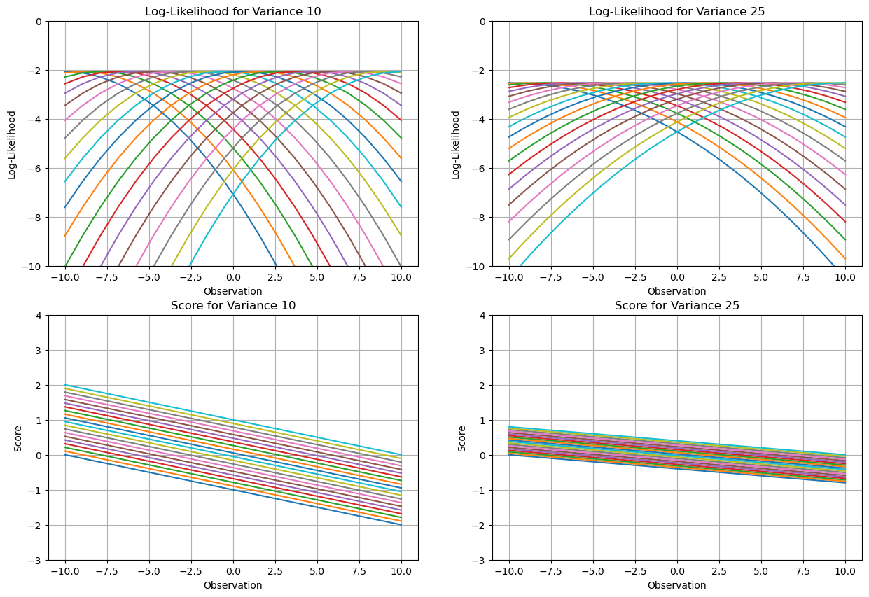
variance1 = 10
variance2 = 25

fig, ((ax1, ax2), (ax3, ax4)) = plt.subplots(2, 2, figsize=(15, 10))


for i, x in enumerate(x_values):
    log_likelihood1 = -0.5 * \
        np.log(2 * np.pi * variance1) - ((x - x_values) ** 2) / (2 * variance1)
    log_likelihood2 = -0.5 * \
        np.log(2 * np.pi * variance2) - ((x - x_values) ** 2) / (2 * variance2)
    score1 = (x - x_values) / variance1
    score2 = (x - x_values) / variance2

    ax1.plot(x_values, log_likelihood1, label=f"Observation Point {i+1}")
    ax2.plot(x_values, log_likelihood2, label=f"Observation Point {i+1}")
    ax3.plot(x_values, score1, label=f"Observation Point {i+1}")
    ax4.plot(x_values, score2, label=f"Observation Point {i+1}")

ax1.set_xlabel("Observation")
ax1.set_ylabel("Log-Likelihood")
ax1.set_title(f"Log-Likelihood for Variance {variance1}")
ax1.grid()
ax1.set_ylim([-10, 0])  # set y-limits

ax2.set_xlabel("Observation")
ax2.set_ylabel("Log-Likelihood")
ax2.set_title(f"Log-Likelihood for Variance {variance2}")
ax2.grid()
ax2.set_ylim([-10, 0])  # set y-limits

ax3.set_xlabel("Observation")
ax3.set_ylabel("Score")
ax3.set_title(f"Score for Variance {variance1}")
ax3.grid()
ax3.set_ylim([-3, 4])
ax4.set_xlabel("Observation")
ax4.set_ylabel("Score")
ax4.set_title(f"Score for Variance {variance2}")
ax4.grid()
ax4.set_ylim([-3, 4])

plt.show()

We see that in the case of less variance the score matrix is more varied and hence contains more information about the true mean. We can also see from the log likliehood graphs that a lower variance is showing us that most points in our sample peak at zero indicating its the true mean wheareas a higher variance does not easily tell us where the peak us.

To make it more intuitive, in our previous example if we can crudely say that when the results follow a ‘pattern’ and the results are less varied we actually have more information about the biasing.